Analysis tools – part 2

I use Mathematica as my swiss army knife for math, data analysis and modeling.

Mathematica can read and write many common file formats, so it’s easy for example to import an audio file to run a Fourier analysis or to compute some coefficients and export them for inclusion in some C/C++ code.

One of its strengths is the ability to perform symbolic computations, although for complex problems it’s often necessary to fall back to numerical methods.

Even more than for solving problems, I love to use it to study data and possible models and to get a better intuitive understanding of known results.
This screenshot shows some calculations I did to help me understand the effect of the feedback delay in a possible digital implementation of a resonant digital filter:

It’s possible to write programs in Mathematica, but they are typically slow. For serious number crunching, over time I have built a small collection of C/C++ routines for generic function optimization. I’ve used them for digital filter design, and I plan to use them for fine tuning the shape of the nonlinear distortion in the CEM filter emulation.

SPICE is an electronic circuit simulator. It’s very useful to understand how analog synth components work. One of the goals of virtual analog synth simulation is to recreate the waveforms generated by the original analog electronics. SPICE can take the schematics and derive by numeric computation the behavior of the circuits. Usually the main characteristics of the actual circuit output will be present also in the digital simulation, and it’s possible to study the signals by inserting probes at various stages along the signal path. SPICE can also show how the circuit’s behavior varies with temperature.

Here is a very simple example circuit of the output stage of the Matrix 1000:

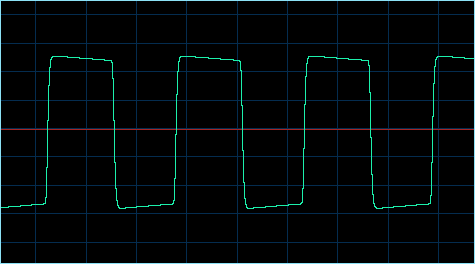
I drew it because when I first looked at a recording of a square wave, it was obvious from the graph that the horizontal segments of the square wave are not horizontal at all (the vertical lines aren’t straight, either, because in the Matrix 1000 it’s not possible to completely disable the low pass filter and because of other effects of the analog circuitry). The horizontal lines have the shape of exponential decay functions, suggesting the presence of a high pass filter:

I was curious to understand how much of the high pass filtering was due to the DC-removal filter on the synth output versus other circuits like the oscillator itself, electronics inside the CEM chip and DC-removal in the audio card). The SPICE simulation of the output stage shows a filter cutoff frequency of about 3 Hz (actual value depends on the input impedance of the audio interface connected to the synth output). The following graph shows the frequency response (red for magnitude, green for phase) of the output stage:

In theory it should be possible to create a virtual analog emulation based on the original circuit and simulating its behavior numerically like SPICE does. However, there are also some major issues with this approach:

• The simulation is expensive in terms of CPU usage. Generous oversampling would also be necessary to limit aliasing.
• The result is only as good as the model used for each electronic component. A look at the graphs on actual datasheets shows that the typical math formulas used in standard models are a good approximation, but typically not a 100% match. It’s possible to get closer by creating more complex models containing many subparts, but this further increases the complexity. For example, one could model all the components that are inside an opamp rather than using simplified formulas, but there may be over one hundred basic components in it, often with unknown specs, and in turn each transistor, capacitor and resistor might need modeling of its non-ideal real-world behavior.
• The model has hundreds of variables, and an error in just one of them can result in inaccuracies.
• Real circuits don’t have all components perfectly matched like in SPICE circuits due to component tolerances and variable temperatures. Good design of the original and thermal-matched components limit the impact of these imperfections, but it is known that some of these effects actually contribute to the warmth of analog sound.
• If the virtual analog implementation contains a very precise representation of the original analog circuit, some could argue that it partially makes use of the intellectual property of the original.

In the case of the CEM 3396 chip that generates each Matrix voice, as far as I know there are no schematics for what’s inside the chip, so SPICE simulation is not feasible. However, I still plan to look at other discrete designs from those years that are probably similar to understand their main characteristics. For example, I don’t currently know why the distortion in the CEM filter is asymmetrical (this is visible in the shape and spectrum of the self-oscillation waveform) and I hope that SPICE experiments can provide me an insight.

Patch map

The following image shows the 1000 patches of the Matrix-1000, each represented by a small colored square. There are 50 squares per row, so each bank is two rows.

Red squares are patches that either use filter modulation or have a click. These are likely the last features that I will try to simulate.

White square patches have a noise component in them. Most of them are in the “FX & Perc” bank.

Yellow patches use only square wave DCOs, blue patches use only the variable waveform, and green patches use both square and waveform DCOs.

This patch map suggests that it should be possible to simulate most patches even before implementing filter modulation, and that I may be able to simulate up to one fourth of the patches (there are 250 yellow squares) after implementing the square wave, the filter and digital control (including envelopes, LFOs and matrix modulation).

It’s also interesting to note that there are two black squares. These correspond to patches with no oscillators and no noise. How is it possible for these patches to produce sound then? The two patches are called heart and zap and loading them in an editor shows that their filter resonance is set to the maximum possible value, so these patches are using the ability of the filter to self-oscillate and produce a sinusoidal output even when it has no input signal.

[tag: 55QSB2593CDW]

Analysis tools – part 1

Studying sounds with enough detail to allow writing a model that can reproduce them means first of all measuring those sounds.

I don’t have expensive lab hardware, but I think a good audio card and some code is all that’s needed. After all, recording tracks with a computer is one of the first steps in any music production that uses a digital audio workstation.

I’m surprised when I read that some virtual analog emulations have been created without access to the original machine, but only based on sound clips recorded by other people. For this project I’ve already collected many thousands of clips, which would be impossible to do without having the synth with me. Maybe the difference is that the goal of those projects was “only” to get the sound right, while I’d also like to reproduce the relationship between the sounds and the patch parameter values (sound generation in the Matrix-1000 is analog, but the sound parameters are digitally controlled and have precise numeric values).

Due to the large number of recordings I plan to take and analyze, acquiring the samples in an audio program and saving the files manually would be impractical, so the first thing I did when I started this project was to write some code to record sound from the audio card, analyze it and save the analysis results for further processing.

As a starting point, I used the code of the CaptureSound code sample in an old DirectX SDK and as an exercise modified it into a Sound Scope application, showing the waveform that the synth is outputting in real time.

The screenshot shows the program’s window, the sound waveform is in the upper half, while the lower half only shows an implementation detail of how the sound’s auto-correlation graph is used to detect the instantaneous sound frequency.

This first code building block was then expanded to an application that can send MIDI patches to the Matrix-1000 - slowly varying selected parameters - and record the sounds resulting from each parameter variation. I can start the application before going to sleep, it will go on all night recording parameter sweeps and in the morning I’ll find one or more files full of juicy data awaiting me.

What to do with all these data? First, a good idea is to graph them, check that they make sense and get an intuitive feeling for how the synth parameters work.

For example, the following graph shows the spectrum of the sound resulting from sending the noise generator output through the low pass filter, for different values of the filter cutoff frequency (this is a logarithmic graph, x is octaves and y is dB):

From these graphs it’s possible for example to measure the cutoff frequency (actual value in Hertz) corresponding to the values indicated in the MIDI SysEx describing the patch. It’s also possible to design a digital filter approximating the analog filter to the desired degree of accuracy.

Studying the data sometimes results in peculiar discoveries (for example, in the above graph it can be seen that when the parameter value is incremented from an odd number to the next (even) number, the actual cutoff frequency increases much less than when the value is incremented from an even number to the next (odd) number), exposes the occasional bug in the synth implementation and often generates even more questions than it answers (for example, is the hump in the graph corresponding to the low frequencies a characteristic of the random noise generator, of the filter response, an artifact or error of the analysis process, or something else entirely?).

The measured data needs some further processing to generate parameters and code that can be used to reproduce the measured quantities in a digital simulation of the synthesizer. Often I will look for a continuous function that approximates the measurements. The following graph shows the measurements of the sound amplitude for each value of the VCA patch parameter (the little diamonds), and a continuous curve that approximates the measured values almost perfectly. The approximation function used in this case is a logistic curve and the values of the curve parameters that best match the experimental data were computed using the Lab Fit software. The result is a mathematical formula that can be used in the virtual analog simulation:

In part 2, I’ll mention a couple of the math and modeling tools I use.

Under the hood

What’s inside the beast? Take a peek:

Let’s take a closer look at the anatomy of this analog synthesizer with a digital brain…

The Oberheim Matrix-1000 is controlled by a 68B09 CPU that handles the UI, processing of MIDI commands and the the envelopes, ramps, LFOs and matrix modulations for all voices.

The 96 KB ROM comes in two chips, one for the operating system (latest version is 1.11) and the other for the 800 preset sounds. The static RAM holds the 200 user-modifiable sounds, global parameters and temporary data used by the operating system at runtime.

The TIMERS block has 4 chips to generate the frequencies for the 12 oscillators (two oscillators for each voice), another timer chip to generate periodic interrupts for the CPU, and the ACIA chip used for MIDI serial communication.

The DAC block contains the 12-bit DAC (it’s the IC at center top in the DAC block) which converts the digital control signals from the CPU to analog signals. The CPU is only 8-bit, a couple of ICs take care of assembling the 12-bit value (plus two extra control bits) for the DAC. Other ICs in this block are demultiplexers. Together with other demultiplexers located in each voice block, they are used to route the analog signal from the single DAC to one of the 60 analog control signals (10 for each voice).

There are six identical circuits for each of the six voices. They are essentially the same as the ones in the Matrix-6.

At the heart of the synth are the six CEM 3396 analog ICs produced by Curtis Electromusic, each one a monophonic synthesizer on its own. The specs include two oscillators, amplifiers and a 4-pole low pass filter with resonance control. The oscillator waveform can be a square wave with variable pulse width or a variety of shapes in between a sawtooth and a triangle. The filter can self-oscillate and has a “filter FM” option.

Around each CEM 3396 chip there are some supporting components, two analog demultiplexers (already mentioned) and a fourth IC dedicated for the most part to implementing oscillator sync. Many of the capacitors in this area are used to optionally smooth the analog control signals.

Status (Feb 2012)

I started this project in 2004, but haven’t worked on it since 2006… let’s see if I can find the time to continue it!

First step is to study the synth sound and how the patch parameters affect it. Second step is to simulate it in software. If this is ever completed, the final step is to package it in something usable (e.g. a VST instrument), add the UI and optimize the code.

Each of the Matrix 1000 voices is generated by the CEM 3396 analog chip, while the sound parameters, envelopes, MIDI and matrix modulation are controlled digitally by the synth’s CPU.

For the core voice emulation, here are some of the things that need to happen before the simulation is complete (green means I completed this part, yellow that I’ve started working on it, red means I haven’t tackled it, yet):

Analog part:

• VCA (volume): characterize amplitude (“characterize” := study how measured quantity depends on inputs and parameters)
• DCO (oscillator): alias-free simplified implementation
• DCO: characterize square waveform timbre
• DCO: characterize sawtooth / triangle waveform timbre
• DCO: characterize noise
• DCO: oscillator sync
• DCO: click
• VCF (filter): characterize filter frequency
• VCF: characterize resonance
• VCF: model non-linearities
• VCF: self-oscillation and variability
• VCF: study filter modulation
• Study voice variability

Digital part:

• Characterize envelopes
• Characterize ramps
• Characterize “tracking” control
• Measure LFO frequencies
• Study “random” LFO
• Characterize matrix modulation (all permutations, there’s a LOT of different cases!)
• Characterize portamento
• Characterize global parameters like vibrato

Hmmm, more red than I’d like…

I can probably get a first set of useable basic sounds after I complete the square wave and filter resonance (including non-linearities). The rest can be added later.

Oberheim Matrix 1000 softsynth project

This blog is about a project to replace the Oberheim Matrix 1000 synthesizer in my rack with a software emulation.